How to Unpivot Messy Spreadsheet Data in Power Query

- Unpivoting converts a wide table into a long table: It changes many columns into few columns and many rows — the normalized shape Power BI's VertiPaq storage engine and Star Schema relationships require.
- Three unpivot choices in Power Query: Unpivot Columns, Unpivot Other Columns, and Unpivot Only Selected Columns. They look identical on initial run, but behave drastically differently when new months or categories arrive at refresh.
- Always prefer "Unpivot Other Columns": By selecting fixed identifier keys (such as Product or Region) and unpivoting the rest, newly added monthly columns get unpivoted automatically without query errors.
- Clean messy rows before unpivoting: Title rows, blank rows, and summary totals must be eliminated before triggering the unpivot step; otherwise, they corrupt your aggregations and double-count numbers.
- Direct M Code control:
Table.UnpivotOtherColumnsprovides predictable, high-speed execution that can be edited in the Advanced Editor when UI controls feel restrictive.
If you've ever imported a monthly report from Excel and found a column for every month instead of a Month column and a Value column, you've hit the classic spreadsheet structure problem. It looks readable to a human. It's nearly useless for Power BI. Unpivoting is the fix — and this guide covers every variation of it, from a clean simple table to the genuinely messy spreadsheets that arrive from real accounting systems and shared drives.
Why Unpivoting Matters: Wide vs Long Format
Before touching Power Query, it's worth understanding exactly why this reshaping is necessary — because knowing why makes the steps make more sense.
A wide table has one row per entity and spreads a repeating dimension (like months) across multiple columns. It's easy to read as a spreadsheet. It's structurally broken for BI work, because there's no single column to filter by month, no way to create a time intelligence measure, and no clean relationship to a Calendar table.
A long table has one row per combination of entity and dimension value — one row for Laptop in January, another for Laptop in February, and so on. It's harder to read as a spreadsheet. It's exactly what Power BI's data model expects.
Here's the same data in both formats. This is the transformation every example in this guide works toward:
Before (Wide — 4 rows, 5 columns):
| Product | Jan 2026 | Feb 2026 | Mar 2026 | Apr 2026 |
|---|---|---|---|---|
| Laptop | 45,000 | 52,000 | 48,000 | 61,000 |
| Mouse | 3,200 | 2,900 | 3,600 | 4,100 |
| Monitor | 28,000 | 31,000 | 29,500 | 33,000 |
| Keyboard | 8,500 | 7,800 | 9,200 | 10,500 |
After (Long — 16 rows, 3 columns):
| Product | Month | Revenue |
|---|---|---|
| Laptop | Jan 2026 | 45,000 |
| Laptop | Feb 2026 | 52,000 |
| Laptop | Mar 2026 | 48,000 |
| Laptop | Apr 2026 | 61,000 |
| Mouse | Jan 2026 | 3,200 |
| … | … | … |
4 rows × 4 month columns = 16 rows. Same data, completely different shape, and now directly usable in Power BI for time intelligence, slicers, and relationship to a Calendar table.
The Three Unpivot Options: What They Are and When to Use Each
Power Query gives you three ways to unpivot columns, and the difference between them is more important than most guides explain. All three produce the same output when you first run them. They behave very differently the next time your data refreshes.
Option 1: Unpivot Columns
You select the columns you want to convert into rows, and Power Query turns exactly those columns — and only those columns — into attribute-value pairs. If a new month column appears in your data next month, it won't be unpivoted automatically. Power Query will treat it like a regular column and leave it wide.
When to use it: When the columns you're unpivoting are permanently fixed and will never change. Rare in real-world spreadsheet work.
= Table.Unpivot(Source, {"Jan 2026", "Feb 2026", "Mar 2026", "Apr 2026"}, "Month", "Revenue")
The column names are hardcoded. If "May 2026" appears next refresh, it stays as a separate column.
Option 2: Unpivot Other Columns
You select the columns you want to keep (the anchor columns — like Product), and Power Query unpivots everything else. This is the future-proof version. When a new month column arrives next refresh, it gets unpivoted automatically without any changes to your query.
When to use it: Almost always. If your column headers represent repeating values (months, years, quarters, products, regions) that will likely grow over time, this is the right option.
= Table.UnpivotOtherColumns(Source, {"Product"}, "Month", "Revenue")
Only "Product" is hardcoded. Every other column gets unpivoted, now and in every future refresh.
Option 3: Unpivot Only Selected Columns
You select the columns you want to unpivot, same as Option 1, but Power Query's behavior is slightly different internally. In current Power BI Desktop, this option works cleanly — it unpivots exactly the columns you selected, and leaves any new columns as-is. It's functionally the same as Option 1 in most scenarios.
When to use it: When you specifically want to unpivot a defined set of columns and leave other non-identifier columns untouched. Useful when your table has both columns-to-keep and columns-to-ignore alongside the ones to unpivot.
Part 1: Unpivoting a Clean Wide Table (The Basic Case)
Start here even if your data is messy — understanding the clean case makes the messy variations easier to follow.
Step 1: Load Your Data Into Power Query
In Power BI Desktop, go to Home → Transform Data to open Power Query Editor. If you're starting fresh, click Home → Get Data → Excel Workbook (or whichever source your data comes from), select your file, choose the correct sheet in the Navigator dialog, and click Transform Data rather than Load.
You should see your wide table in the Power Query preview pane — one row per product, one column per month.

Step 2: Identify Your Anchor Columns
Before touching anything, identify which columns are identifiers (things that should stay as columns) and which are values (things that should become rows). In the sample table:
- Anchor/identifier: Product — this stays as a column
- Values to unpivot: Jan 2026, Feb 2026, Mar 2026, Apr 2026 — these become rows
This distinction is what determines which unpivot option you choose and what you select before clicking it.
Step 3: Select the Anchor Column and Unpivot Other Columns
Click the Product column header to select it. This is the column you're keeping — not the one you're unpivoting.
Right-click the selected column header. In the context menu, you'll see three options:
- Unpivot Columns
- Unpivot Other Columns ← click this one
- Unpivot Only Selected Columns
Select Unpivot Other Columns. Alternatively, with the Product column selected, go to the Transform tab in the ribbon and use the Unpivot Columns dropdown there. The same three options appear.

Step 4: Review the Result
Power Query immediately reshapes the table. What was a 4-row, 5-column table is now a 16-row, 3-column table. Two new columns appear:
- Attribute: contains the former column headers (Jan 2026, Feb 2026, etc.)
- Value: contains the numbers that were under each column header
The data is correct. The column names aren't — "Attribute" and "Value" are Power Query's generic defaults, and you need to rename them immediately.
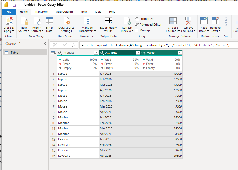
Step 5: Rename the Attribute and Value Columns
Double-click the Attribute column header and rename it to Month (or whatever the column headers actually represented — Year, Quarter, Region, Category, etc.).
Double-click the Value column header and rename it to Revenue (or Sales, Units, Amount — whatever the numbers represent).
This step is easy to forget and important to do before closing the query, because these names become your field names in the Power BI data model. "Attribute" appearing as a field in your report is a sign the cleanup wasn't finished.

Step 6: Set the Correct Data Types
Click the small icon at the left edge of each column header to see and change the data type:
- Product column: Text ✓ (usually already correct)
- Month column: If your headers were proper dates formatted as "Jan 2026," Power Query may keep them as text. You have two options: convert the text to a Date type using the data type icon, or leave it as text and link to a dedicated Date dimension.
- Revenue column: Whole Number or Decimal Number — not Text. Click the icon and select the correct numeric type.
Setting data types wrong here — especially leaving Revenue as text — is the most common cause of measures returning errors or blanks after an unpivot.
Step 7: Review the Applied Steps
Look at the Applied Steps panel on the right side. You should see steps like:
If any step shows an error indicator (a small warning icon), click it to see what went wrong before proceeding.
Step 8: Close and Apply
Click Home → Close & Apply. Power Query loads the reshaped table into your Power BI data model. You can now connect it to a Calendar table using the Month (Date) column, create measures that aggregate Revenue, and build time-intelligence calculations that wouldn't have been possible against the original wide table.
Part 2: Cleaning Up a Messy Spreadsheet Before Unpivoting
Real spreadsheets from accounting systems, shared drives, and email attachments rarely arrive as clean tables. More often they look like this:
Power Query imports everything — title rows, blank rows, summary rows, all of it. The cleanup has to happen before the unpivot. Here's the correct sequence.
Step 1: Import the File and Open Power Query
Get Data → Excel Workbook → select your file → in the Navigator, select the sheet → click Transform Data (not Load). Power Query shows you the raw import. The first row is the title. Column headers read "Column1, Column2, Column3..." because the real headers are buried further down.
Step 2: Remove the Title Row(s)
Go to Home → Remove Rows → Remove Top Rows. Enter the number of rows to remove — in this example, 2 (the title row and the blank row beneath it). Click OK.
Now the first row of the preview contains your real column headers (Product, Jan 2026, Feb 2026, etc.), but they're still sitting in the data as a row, not recognized as headers yet.
Step 3: Promote the First Row to Headers
Go to Home → Use First Row as Headers (or Transform → Use First Row as Headers). Power Query promotes the first data row into column names. Your columns now have the right names.
Step 4: Remove Blank Rows
Go to Home → Remove Rows → Remove Blank Rows. This removes any fully empty rows. If rows are only partially blank (some cells empty but not all), filter those out manually — click the dropdown arrow on a key column like Product and uncheck the blank/null option.
Step 5: Remove Summary or Total Rows
If your spreadsheet had a "Total" row at the bottom (or a "Grand Total" row partway through), filter it out. Click the dropdown arrow on the Product column and uncheck "Total" (or whatever label the summary row uses). This is critical — if you leave a Total row in and unpivot it, the totals become data points that double-count your actual numbers when you build measures.
Step 6: Fix Data Types for Any Numeric Columns That Came in as Text
When Power Query imports a messy spreadsheet, numbers often come in as text — especially if the spreadsheet used formatted cells with currency symbols or thousand separators. Before unpivoting, check each numeric column and change its type to Whole Number or Decimal Number if it currently shows as Text or Any.
Step 7: Now Unpivot (Following the Clean Table Steps Above)
With the messy data now cleaned up, follow Steps 2 through 8 from Part 1. Select the Product column, right-click, choose Unpivot Other Columns, rename Attribute and Value, set data types, and close and apply.
The order matters here and is worth being explicit about: clean first, unpivot second. Trying to unpivot before removing title rows, blank rows, and summary rows produces a garbled result that's harder to fix than starting the cleanup from scratch.
Part 3: Unpivoting When You Have Multiple Value Columns Per Period
A harder scenario that trips up even experienced Power Query users: your data has two (or more) measurements per period, stored as separate columns per period.
Example — Revenue and Quantity per month:
| Product | Jan_Revenue | Jan_Qty | Feb_Revenue | Feb_Qty |
|---|---|---|---|---|
| Laptop | 45,000 | 15 | 52,000 | 17 |
| Mouse | 3,200 | 160 | 2,900 | 145 |
You can't run a single unpivot here and get a clean result, because you have two different types of values mixed together. A plain unpivot would give you rows where Attribute is "Jan_Revenue" and others where it's "Jan_Qty" — technically unpivoted, but not cleanly separated into distinct columns.
The correct approach is to unpivot and then split the Attribute column to separate the period from the measure type:
Step 1: Unpivot All Value Columns
Select the Product column, right-click, Unpivot Other Columns. You get a long table with Attribute values like "Jan_Revenue," "Jan_Qty," "Feb_Revenue," "Feb_Qty."
Step 2: Split the Attribute Column by Delimiter
Select the Attribute column. Go to Transform → Split Column → By Delimiter. Choose the underscore _ as the delimiter, split at the leftmost delimiter (so "Jan_Revenue" splits into "Jan" and "Revenue"). Click OK. Power Query creates two columns: Attribute.1 (the period) and Attribute.2 (the measure name).
Step 3: Rename the Split Columns
Rename Attribute.1 to Month and Attribute.2 to Measure.
Step 4: Pivot the Measure Column Back
Now you have a long table with Month, Measure (Revenue or Qty), and Value. To get Revenue and Qty as separate columns (which is usually more useful for modeling), select the Measure column and go to Transform → Pivot Column. Set the values column to Value and the aggregation to Don't Aggregate (or Sum if there are duplicates). Click OK.
The result is a clean table with Product, Month, Revenue, and Qty as separate columns — exactly the shape you wanted.
Part 4: The M Code Behind Unpivot
Every step Power Query takes through the UI is recorded as M code. For most unpivot scenarios, you never need to touch the M code directly. But knowing what it looks like — and how to edit it — gives you a safety net when the UI doesn't quite do what you need.
Click Home → Advanced Editor in Power Query to see the full M code for your query. For the basic unpivot from Part 1, it looks like this:
let
    Source = Excel.Workbook(File.Contents("C:\Data\SalesData.xlsx"), null, true),
    Sheet1_Sheet = Source{[Item="Sheet1",Kind="Sheet"]}[Data],
    #"Promoted Headers" = Table.PromoteHeaders(Sheet1_Sheet, [PromoteAllScalars=true]),
    #"Changed Type" = Table.TransformColumnTypes(#"Promoted Headers",{
        {"Product", type text},
        {"Jan 2026", Int64.Type},
        {"Feb 2026", Int64.Type},
        {"Mar 2026", Int64.Type},
        {"Apr 2026", Int64.Type}
    }),
    #"Unpivoted Other Columns" = Table.UnpivotOtherColumns(
        #"Changed Type",
        {"Product"},
        "Month",
        "Revenue"
    ),
    #"Changed Type1" = Table.TransformColumnTypes(#"Unpivoted Other Columns",{
        {"Month", type text},
        {"Revenue", Int64.Type}
    })
in
    #"Changed Type1"
The key line is Table.UnpivotOtherColumns. The arguments are:
#"Changed Type"— the previous step's output (the table to unpivot){"Product"}— the list of columns to keep as identifiers"Month"— the name for the new Attribute column"Revenue"— the name for the new Value column
If you need to add a second anchor column — say your table has both Product and Region as identifiers — you just add it to the list: {"Product", "Region"}.
For the hardcoded version (Unpivot Only Selected Columns), the M function is Table.Unpivot:
= Table.Unpivot(
    #"Changed Type",
    {"Jan 2026", "Feb 2026", "Mar 2026", "Apr 2026"},
    "Month",
    "Revenue"
)
Part 5: When Unpivot Doesn't Work — Common Errors and Fixes
Error: "We cannot convert the value null to type Number"
Cause: Blank cells in your value columns, which Power Query tries to convert to a number during the Changed Type step and fails.
Fix: Before the unpivot step, go to Transform → Replace Values on each value column. Replace null with 0 (or blank, depending on whether you want zero or blank in your measures). Then run the unpivot.
Error: Expression.Error — The column 'May 2026' of the table wasn't found
Cause: You used Unpivot Only Selected Columns (Option 1 or 3) and hardcoded specific column names. A new column with a different name arrived at refresh.
Fix: Delete the unpivot step from Applied Steps, re-select your anchor columns, and redo the unpivot using Unpivot Other Columns instead. Update the M code if you prefer: replace Table.Unpivot with Table.UnpivotOtherColumns and change the second argument from a list of value columns to a list of your anchor columns only.
Result Has Rows Where Attribute = Column Names From a Header Row
Cause: You promoted headers after the unpivot instead of before it, or a summary/header row survived the cleanup step.
Fix: In Applied Steps, check the order. "Promoted Headers" should appear before "Unpivoted Other Columns." If a header row still exists as data, use Remove Top Rows or a filter step to eliminate it before the unpivot step.
All Values in the Value Column Are Text Instead of Numbers
Cause: The original numeric columns had data type "Any" or "Text" before the unpivot, and the unpivot inherited that type.
Fix: In Applied Steps, find the "Changed Type" step that comes before the unpivot. Click the gear icon next to it and add type assignments for the numeric columns (set them to Int64.Type or type number). Alternatively, after the unpivot, select the Revenue column and use the data type icon to change it to Whole Number — but fixing it before the unpivot is cleaner.
The Attribute Column Contains "Jan 2026", "Feb 2026" as Text, Not Dates
Cause: Month headers stored as text strings can't be auto-converted to dates. Power Query keeps them as text after unpivoting.
Fix: Add a Custom Column step after the unpivot using Date.FromText([Month]) or DateTime.FromText([Month]). If the text format is non-standard (like "Jan-26"), use Date.FromText(Text.Replace([Month], " ", "-1-")) to insert a day before parsing. Alternatively, add a proper date table with a Month label column and use that for the relationship instead of trying to parse the text directly.
In Practice: A Real Scenario
A finance team receives a monthly Excel export from their ERP system. Every export arrives as a new file named Sales_YYYYMM.xlsx, dropped into a SharePoint folder. Each file has the same structure: a title row, a blank row, column headers in row 3, revenue data for four products across twelve months, and a Grand Total row at the bottom.
Using the Folder connector, Power BI connects to the SharePoint folder, combines all files, and runs the transformation steps once against the combined dataset.
The Power Query transformation sequence for this real scenario, in order:
- Remove top 2 rows (title + blank)
- Promote headers
- Remove blank rows
- Filter out "Grand Total" rows from Product column
- Change data types on the month columns to Whole Number
- Unpivot Other Columns (keeping Product as the anchor)
- Rename Attribute → Month, Value → Revenue
- Add a custom column to convert Month text to a proper Date
- Change Revenue column type to Whole Number
- Close and Apply
The finance team drops each new monthly file into the SharePoint folder. The next scheduled refresh runs these ten steps against the updated folder contents automatically, adding the new month's data without anyone touching Power Query. The total hands-on time after the initial setup: zero.
Quick Reference: The Full Unpivot Decision Tree
Is your data wide (values spread across columns)?
    └── YES → Need to unpivot
        ├── Are the column headers values that could grow over time (months, years, regions)?
        │       └── YES → Use UNPIVOT OTHER COLUMNS (select anchor columns, unpivot everything else)
        ├── Are the column headers permanently fixed and will never change?
        │       └── YES → Use UNPIVOT ONLY SELECTED COLUMNS (select value columns to unpivot)
        └── Do you have multiple value types per period (Revenue AND Qty per month)?
                └── YES → Unpivot Other Columns → Split Attribute column → Pivot Measure column back
Frequently Asked Questions
What's the difference between Unpivot Columns and Unpivot Other Columns in Power Query?
Unpivot Columns hardcodes the specific columns you selected — new columns appearing at refresh won't be unpivoted automatically. Unpivot Other Columns hardcodes the columns you want to keep, and unpivots everything else — new columns are automatically included at the next refresh. For most real-world scenarios with growing data, Unpivot Other Columns is the correct choice.
What are the Attribute and Value columns that appear after unpivoting?
Attribute contains the former column headers — the month names, year labels, or whatever the column headers represented. Value contains the numbers that were in those columns. Power Query uses these generic default names. Rename them immediately to match what they actually represent (Month, Revenue, Year, Units, etc.).
Can I unpivot multiple columns at once if they have different meanings?
Not cleanly with a single unpivot operation. If you have Revenue and Quantity both stored as separate columns per month, you need to unpivot all value columns first, then split the Attribute column to separate the measure type from the period, then optionally pivot the measure type back into separate columns.
Why does my unpivot break when new columns arrive at refresh?
Because you used Unpivot Columns or Unpivot Only Selected Columns, which hardcode specific column names. Switch to Unpivot Other Columns — it hardcodes the anchor columns instead of the value columns, making your query self-updating when new value columns appear.
Do I need to clean up messy rows before or after unpivoting?
Before. Title rows, blank rows, and summary rows should be removed before the unpivot step. If they survive into the unpivot, they become data rows in your long table — the "Total" row becomes a Laptop-level data point and corrupts your aggregations.
What's the M code for Unpivot Other Columns?
Table.UnpivotOtherColumns(previousStep, {"AnchorColumn1", "AnchorColumn2"}, "Attribute", "Value") — replace the anchor column list with your actual identifier columns, and replace "Attribute" and "Value" with your preferred output column names.
Recommended Next Guides & Deep Dives
Continue expanding your Power BI and Fabric architecture knowledge with these closely connected tutorials:
-
Power Query M Language for Beginners
→
Inspect the Table.UnpivotOtherColumns function generated in the Advanced Editor.
-
Star Schema vs Snowflake Schema in Power BI
→
Transform wide human-entered spreadsheets into columnar star schema facts.
-
Automate Monthly Excel Folder Imports
→
Unpivot batch files automatically as new spreadsheets arrive each month.
-
Fuzzy Matching in Power Query
→
Clean unpivoted categorical dimensions that contain typos or alias variations.
-
Profit and Loss Dashboard in Power BI
→
Reshape monthly financial trial balances for interactive matrix visuals.

Vivek Dhumal
BI Consultant
BI Consultant & Power BI Developer
Vivek Dhumal is a dedicated BI Consultant and Data Analyst specializing in Power BI development, DAX calculations, SQL data modeling, ETL automation, and scalable business intelligence solutions.